Gather & Spread

Overview

Teaching: 30 min
Exercises: 15 min

Questions

How can I change the format of dataframes?

Objectives

To understand the concepts of ‘long’ and ‘wide’ data formats and be able to convert between them with tidyr.

Having had some exposure to working with tidyverse functions, you might now understand why it is beneficial to work with tidy data. These data manipulation functions are all designed to work easily with tidy data, leaving you with more time to actually try to answer questions with the data.

Unfortunately, real data sets can come in all shapes and sizes and may not be structured for you to efficiently analyse it. To help tidy our data up in preparation for analysis, we will turn to the tidyr package from the tidyverse.

Tidy data review

Before getting into a real example, we’ll have a look at a toy dataset. The following dataframe has two weight measurements for three different cows. Have a look at the way the data is structured. Is it tidy?

cows <- data_frame(id = c(1, 2, 3),
                   weight1 = c(203, 227, 193),
                   weight2 = c(365, 344, 329))
cows

# A tibble: 3 × 3
     id weight1 weight2
  <dbl>   <dbl>   <dbl>
1     1     203     365
2     2     227     344
3     3     193     329

What might make this dataset tidy?

Table massaging with `gather()` and `spread()`

To make this dataframe tidy, we may need to have only one weight variable, and another variable describing whether it is measurement 1 or 2. The gather() function from tidyr can do this conversion for us. You can think of gather() as scooping all the data up into one big tall pile.

cows_long <- cows %>% 
  gather(measurement, weight, weight1, weight2)

cows_long

# A tibble: 6 × 3
     id measurement weight
  <dbl> <chr>        <dbl>
1     1 weight1        203
2     2 weight1        227
3     3 weight1        193
4     1 weight2        365
5     2 weight2        344
6     3 weight2        329

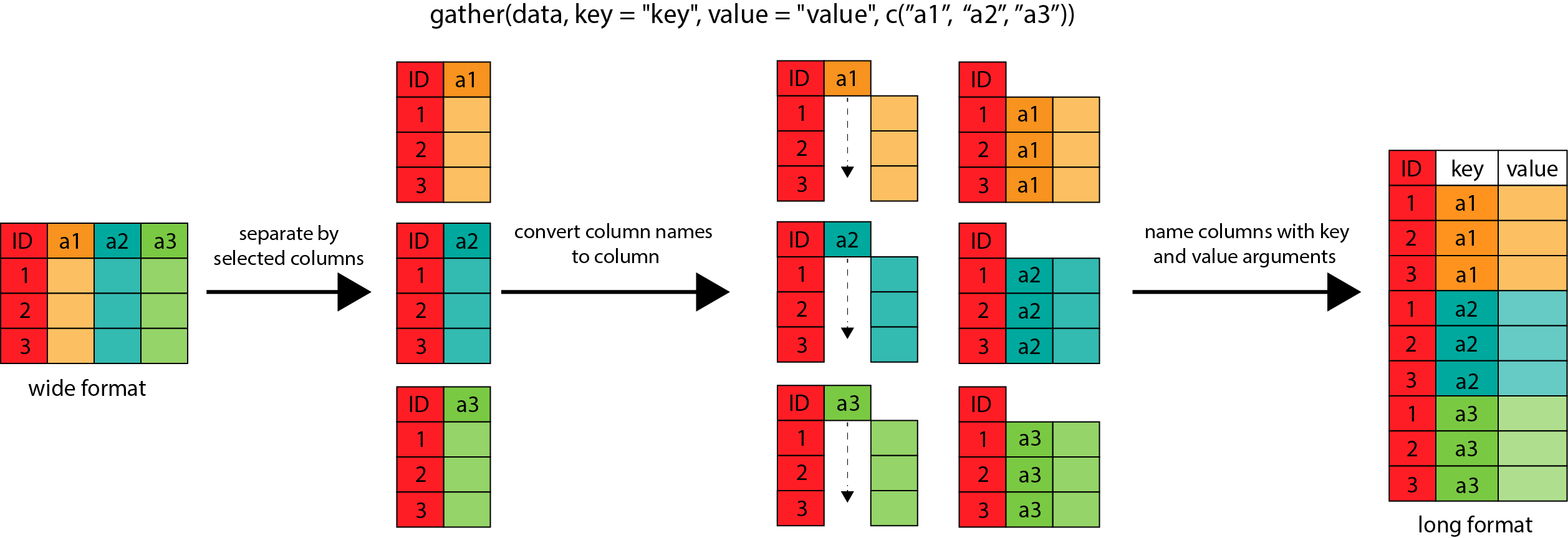
gather() works by converting the data into a set of key-value pairs, in which the key describes what the data is, and the value records the actual data. For example, weight1-203 is the key-value pair for the first row of the gathered table.

The call to gather() therefore works in two parts. First we specify the names of the new key-value pair columns (measurement and weight in this case). Then we tell it which columns should be gathered (weight1 and weight2 here). gather() then takes the contents of those columns and places them into the new value column, and labels them with their column name as the key.

This transformation may be easier to see in action, so let’s have a look at the way gather() has worked on the original data.

As well as going from wide to long, we can go back the other way. Instead of gather(), we need to spread() the data.

cows_long %>% 
  spread(measurement, weight)

# A tibble: 3 × 3
     id weight1 weight2
  <dbl>   <dbl>   <dbl>
1     1     203     365
2     2     227     344
3     3     193     329

This works in reverse, taking the names of out key-value columns and spreading them out. Each unique value in the key column is given a separate column of it’s own. And the content of that column is taken from the specified value column.

Realistic data

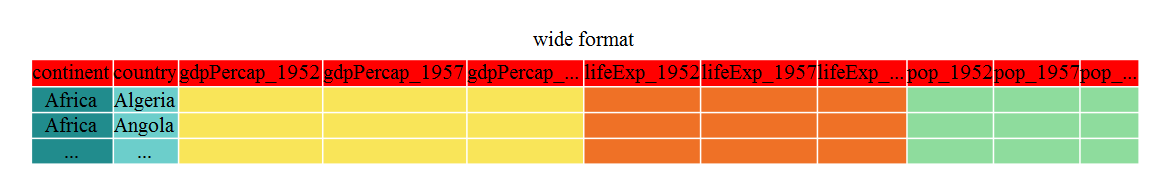
Until now, we’ve been using the original gapminder dataset which comes pre-tidied, but ‘real’ data (i.e. our own research data) will never be so well organised. Here let’s start with the wide format version of the gapminder dataset.

Download the wide version of the gapminder data from here and save it in your project’s data directory.

Read in the wide gapminder and have a look at it.

gap_wide <- read_csv("data/gapminder_wide.csv")

gap_wide

# A tibble: 142 × 38
   continent country gdpPercap_1952 gdpPercap_1957 gdpPercap_1962 gdpPercap_1967
   <chr>     <chr>            <dbl>          <dbl>          <dbl>          <dbl>
 1 Africa    Algeria          2449.          3014.          2551.          3247.
 2 Africa    Angola           3521.          3828.          4269.          5523.
 3 Africa    Benin            1063.           960.           949.          1036.
 4 Africa    Botswa…           851.           918.           984.          1215.
 5 Africa    Burkin…           543.           617.           723.           795.
 6 Africa    Burundi           339.           380.           355.           413.
 7 Africa    Camero…          1173.          1313.          1400.          1508.
 8 Africa    Centra…          1071.          1191.          1193.          1136.
 9 Africa    Chad             1179.          1308.          1390.          1197.
10 Africa    Comoros          1103.          1211.          1407.          1876.
# ℹ 132 more rows
# ℹ 32 more variables: gdpPercap_1972 <dbl>, gdpPercap_1977 <dbl>,
#   gdpPercap_1982 <dbl>, gdpPercap_1987 <dbl>, gdpPercap_1992 <dbl>,
#   gdpPercap_1997 <dbl>, gdpPercap_2002 <dbl>, gdpPercap_2007 <dbl>,
#   lifeExp_1952 <dbl>, lifeExp_1957 <dbl>, lifeExp_1962 <dbl>,
#   lifeExp_1967 <dbl>, lifeExp_1972 <dbl>, lifeExp_1977 <dbl>,
#   lifeExp_1982 <dbl>, lifeExp_1987 <dbl>, lifeExp_1992 <dbl>, …

You can see that wide format has many more columns than our original gapminder data because each metric has a separate column for each year of measurement.

From wide to long

The first step towards recreating the nice and tidy gapminder format is to convert this data from a wide to a long format. The tidyr function gather() will ‘gather’ your observation variables into a single variable.

gap_long <- gap_wide %>%
    gather(obstype_year, obs_values, starts_with('pop'),
           starts_with('lifeExp'), starts_with('gdpPercap'))
gap_long

# A tibble: 5,112 × 4
   continent country                  obstype_year obs_values
   <chr>     <chr>                    <chr>             <dbl>
Africa    Algeria                  pop_1952        9279525
Africa    Angola                   pop_1952        4232095
Africa    Benin                    pop_1952        1738315
Africa    Botswana                 pop_1952         442308
Africa    Burkina Faso             pop_1952        4469979
Africa    Burundi                  pop_1952        2445618
Africa    Cameroon                 pop_1952        5009067
Africa    Central African Republic pop_1952        1291695
Africa    Chad                     pop_1952        2682462
Africa    Comoros                  pop_1952         153936
# ℹ 5,102 more rows

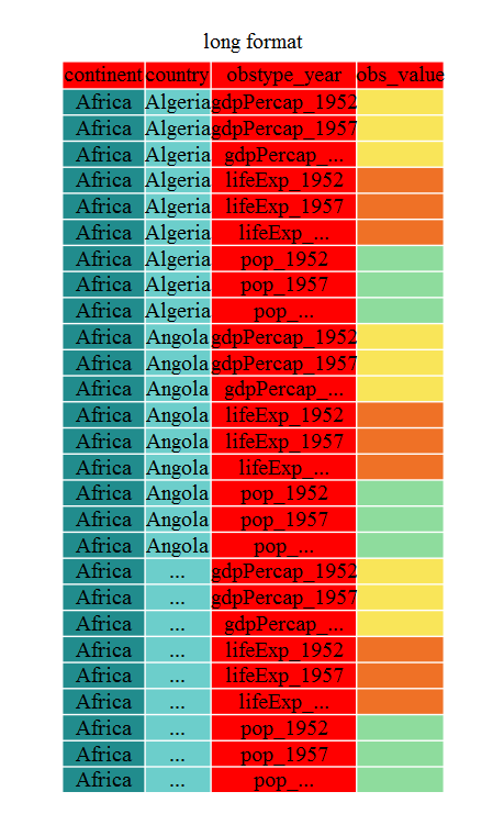
Inside gather() we first name the new column for the new ID variable (obstype_year), the name for the new amalgamated observation variable (obs_value), then the names of the old observation variable. We could have typed out all the observation variables, but since gather() can use all the same helper functions as the select() function can, we can use the starts_with() argument to select all variables that starts with the desired character string. Gather also allows the alternative syntax of using the - symbol to identify which variables are not to be gathered (i.e. ID variables) so that

gap_long <- gap_wide %>% 
  gather(obstype_year, obs_values, -continent, -country)

is an alternative way of specifying the columns to gather in the wide data set. The best method for any particular data set will depend on how many columns you need to gather and how they are named.

Separating column data

Now, the obstype_year column actually contains two pieces of information, the observation type (pop,lifeExp, or gdpPercap) and the year. We can use the separate() function to split the character strings into multiple variables.

gap_separated <- gap_long %>% 
  separate(obstype_year, into = c('obs_type', 'year'), sep = "_")

gap_separated

# A tibble: 5,112 × 5
   continent country                  obs_type year  obs_values
   <chr>     <chr>                    <chr>    <chr>      <dbl>
Africa    Algeria                  pop      1952     9279525
Africa    Angola                   pop      1952     4232095
Africa    Benin                    pop      1952     1738315
Africa    Botswana                 pop      1952      442308
Africa    Burkina Faso             pop      1952     4469979
Africa    Burundi                  pop      1952     2445618
Africa    Cameroon                 pop      1952     5009067
Africa    Central African Republic pop      1952     1291695
Africa    Chad                     pop      1952     2682462
Africa    Comoros                  pop      1952      153936
# ℹ 5,102 more rows

You provide separate() with a column name containing the values to split, the names of the columns you would like to separate them into, and where to split the values (by default it splits on any non alphanumeric character).

Challenge 1

If you look at the table above, you will see that separate() creates character columns out of both the obs_type and year columns, but our original gapminder has year as a numeric. How would you fix this discrepancy?

Hint: Read through the arguments for separate with ?separate

Solution to Challenge 1

The convert argument will try to convert character strings to other data types when set to TRUE

gap_separated <- gap_long %>% 
  separate(obstype_year, into = c('obs_type', 'year'), sep = "_", convert = TRUE)

gap_separated

# A tibble: 5,112 × 5
   continent country                  obs_type  year obs_values
   <chr>     <chr>                    <chr>    <int>      <dbl>
Africa    Algeria                  pop       1952    9279525
Africa    Angola                   pop       1952    4232095
Africa    Benin                    pop       1952    1738315
Africa    Botswana                 pop       1952     442308
Africa    Burkina Faso             pop       1952    4469979
Africa    Burundi                  pop       1952    2445618
Africa    Cameroon                 pop       1952    5009067
Africa    Central African Republic pop       1952    1291695
Africa    Chad                     pop       1952    2682462
Africa    Comoros                  pop       1952     153936
# ℹ 5,102 more rows

The opposite to separate() is unite(). Use this when you are wanting to combine columns into one long string. You provide unite() with the name to give the newly combined column, and the names of the columns to combine.

gap_separated %>% 
  unite(obstype_year, obs_type, year)

# A tibble: 5,112 × 4
   continent country                  obstype_year obs_values
   <chr>     <chr>                    <chr>             <dbl>
Africa    Algeria                  pop_1952        9279525
Africa    Angola                   pop_1952        4232095
Africa    Benin                    pop_1952        1738315
Africa    Botswana                 pop_1952         442308
Africa    Burkina Faso             pop_1952        4469979
Africa    Burundi                  pop_1952        2445618
Africa    Cameroon                 pop_1952        5009067
Africa    Central African Republic pop_1952        1291695
Africa    Chad                     pop_1952        2682462
Africa    Comoros                  pop_1952         153936
# ℹ 5,102 more rows

From long to tidy

The final step in recreating the gapminder data structure is to spread our observation variables out from the long format we have created.

Challenge 2

Spread the gap_separated data above to create a new data frame that has the same dimensions as the original gapminder data.

Solution to Challenge 2

gap_orig <- gap_separated %>% 
  spread(obs_type, obs_values)

gap_orig

# A tibble: 1,704 × 6
   continent country  year gdpPercap lifeExp      pop
   <chr>     <chr>   <int>     <dbl>   <dbl>    <dbl>
Africa    Algeria  1952     2449.    43.1  9279525
Africa    Algeria  1957     3014.    45.7 10270856
Africa    Algeria  1962     2551.    48.3 11000948
Africa    Algeria  1967     3247.    51.4 12760499
Africa    Algeria  1972     4183.    54.5 14760787
Africa    Algeria  1977     4910.    58.0 17152804
Africa    Algeria  1982     5745.    61.4 20033753
Africa    Algeria  1987     5681.    65.8 23254956
Africa    Algeria  1992     5023.    67.7 26298373
Africa    Algeria  1997     4797.    69.2 29072015
# ℹ 1,694 more rows

dim(gap_orig)

[1] 1704    6

dim(gapminder)

[1] 1704    6

We’re almost there, the original was sorted by country, continent, then year. So finish everything off with an arrange() and then a select() to get the columns in the right order.

gap_orig <- gap_orig %>% 
  arrange(country, continent, year) %>% 
  select(country, continent, year, lifeExp, pop, gdpPercap)

gap_orig

# A tibble: 1,704 × 6
   country     continent  year lifeExp      pop gdpPercap
   <chr>       <chr>     <int>   <dbl>    <dbl>     <dbl>
Afghanistan Asia       1952    28.8  8425333      779.
Afghanistan Asia       1957    30.3  9240934      821.
Afghanistan Asia       1962    32.0 10267083      853.
Afghanistan Asia       1967    34.0 11537966      836.
Afghanistan Asia       1972    36.1 13079460      740.
Afghanistan Asia       1977    38.4 14880372      786.
Afghanistan Asia       1982    39.9 12881816      978.
Afghanistan Asia       1987    40.8 13867957      852.
Afghanistan Asia       1992    41.7 16317921      649.
Afghanistan Asia       1997    41.8 22227415      635.
# ℹ 1,694 more rows

gapminder

# A tibble: 1,704 × 6
   country     continent  year lifeExp      pop gdpPercap
   <chr>       <chr>     <dbl>   <dbl>    <dbl>     <dbl>
Afghanistan Asia       1952    28.8  8425333      779.
Afghanistan Asia       1957    30.3  9240934      821.
Afghanistan Asia       1962    32.0 10267083      853.
Afghanistan Asia       1967    34.0 11537966      836.
Afghanistan Asia       1972    36.1 13079460      740.
Afghanistan Asia       1977    38.4 14880372      786.
Afghanistan Asia       1982    39.9 12881816      978.
Afghanistan Asia       1987    40.8 13867957      852.
Afghanistan Asia       1992    41.7 16317921      649.
Afghanistan Asia       1997    41.8 22227415      635.
# ℹ 1,694 more rows

Great work! We’ve taken a messy data set and tidied it into a form that works well with all the tidyverse functions you have been using up until now.

Challenge 3

Practice your gathering skills with the inbuilt tidyr::table4a data frame, which contains the number of TB cases recorded by the WHO in three countries in 1999 and 2000. Is the data frame untidy, and can you tidy it with gather()?
tidyr::table4a
# A tibble: 3 × 3
  country     `1999` `2000`
  <chr>        <dbl>  <dbl>
1 Afghanistan    745   2666
2 Brazil       37737  80488
3 China       212258 213766
Solution to Challenge 3
gather(tidyr::table4a, key = year, value = TB_cases, -country)
# A tibble: 6 × 3
  country     year  TB_cases
  <chr>       <chr>    <dbl>
1 Afghanistan 1999       745
2 Brazil      1999     37737
3 China       1999    212258
4 Afghanistan 2000      2666
5 Brazil      2000     80488
6 China       2000    213766

Challenge 4

Practice your spreading skills with the inbuilt tidyr::table2 data frame, which contains the number of TB cases recorded by the WHO in three countries in 1999 and 2000 as well as their population. Is the data frame untidy, and can you tidy it with spread()?

tidyr::table2

# A tibble: 12 × 4
   country      year type            count
   <chr>       <dbl> <chr>           <dbl>
Afghanistan  1999 cases             745
Afghanistan  1999 population   19987071
Afghanistan  2000 cases            2666
Afghanistan  2000 population   20595360
Brazil       1999 cases           37737
Brazil       1999 population  172006362
Brazil       2000 cases           80488
Brazil       2000 population  174504898
China        1999 cases          212258
China        1999 population 1272915272
China        2000 cases          213766
China        2000 population 1280428583

Solution to Challenge 4

spread(tidyr::table2, key = type, value = count)

# A tibble: 6 × 4
  country      year  cases population
  <chr>       <dbl>  <dbl>      <dbl>
1 Afghanistan  1999    745   19987071
2 Afghanistan  2000   2666   20595360
3 Brazil       1999  37737  172006362
4 Brazil       2000  80488  174504898
5 China        1999 212258 1272915272
6 China        2000 213766 1280428583

Key Points

Use the tidyr package to change the layout of dataframes.

Use gather() to go from wide to long format.

Use spread() to go from long to wide format.

previous episode

Introduction to R

next episode

Gather & Spread

Overview

Tidy data review

Table massaging with `gather()` and `spread()`

Realistic data

From wide to long

Separating column data

Challenge 1

Solution to Challenge 1

From long to tidy

Challenge 2

Solution to Challenge 2

Challenge 3

Solution to Challenge 3

Challenge 4

Solution to Challenge 4

Key Points

previous episode

next episode

previous episode

Introduction to R

next episode

Gather & Spread

Overview

Tidy data review

Table massaging with gather() and spread()

Realistic data

From wide to long

Separating column data

Challenge 1

Solution to Challenge 1

From long to tidy

Challenge 2

Solution to Challenge 2

Challenge 3

Solution to Challenge 3

Challenge 4

Solution to Challenge 4

Key Points

previous episode

next episode

Table massaging with `gather()` and `spread()`