Adding and Combining Datasets
Overview
Teaching: 30 min
Exercises: 30 minQuestions
How can I combine multiple datasets?
How can I merge datasets that have a common variable?
Objectives
Be able to combine different datasets by row, column or common variable
All the functions we have looked at so far work with a single data frame and modify it in some way. It is common, however, that your data may not be stored in a single, complete, form and instead will be found in a number of places. Perhaps measurements taken in different weeks have been saved to separate places, or maybe you have different files recording observations and metadata. To work with data stored like this it is necessary to learn how to combine and merge different datasets into a single data frame.
Combining data
If you have new data that has the same structure as your old data, it can be added onto the end of
your data frame with bind_rows(). We have collected the gapminder data for 2012
into a separate file for you to practice this with. Download this file and save it in your data
directory as gapminder_2012.csv.
gapminder_2012 <- read_csv("data/gapminder_2012.csv")
Rows: 134 Columns: 6
── Column specification ───────────────────────────────────────────────────────────────────────────────────────────────────────────
Delimiter: ","
chr (2): country, continent
dbl (4): year, lifeExp, pop, gdpPercap

ℹ Use `spec()` to retrieve the full column specification for this data.
ℹ Specify the column types or set `show_col_types = FALSE` to quiet this message.
gapminder_2012
# A tibble: 134 × 6
   country     continent  year lifeExp       pop gdpPercap
   <chr>       <chr>     <dbl>   <dbl>     <dbl>     <dbl>
 1 Afghanistan Asia       2012    57.2  30700000      1840
 2 Albania     Europe     2012    77     2920000     10400
 3 Algeria     Africa     2012    76.8  37600000     13200
 4 Angola      Africa     2012    61.7  25100000      6000
 5 Argentina   Americas   2012    76.1  42100000     19200
 6 Australia   Oceania    2012    82.3  22800000     42600
 7 Austria     Europe     2012    80.9   8520000     44400
 8 Bahrain     Asia       2012    76.3   1300000     41500
 9 Bangladesh  Asia       2012    71.3 156000000      2710
10 Belgium     Europe     2012    80.3  11100000     41000
# ℹ 124 more rows
Challenge 1
Combine the 2012 data with your gapminder data using
bind_rows(gapminder, gapminder_2012).Explore the resulting data frame to see the effect of
bind_rows().Solution to Challenge 1
combined_gapminder <- bind_rows(gapminder, gapminder_2012)

tail(combined_gapminder)
# A tibble: 6 × 6 country continent year lifeExp pop gdpPercap <chr> <chr> <dbl> <dbl> <dbl> <dbl> 1 United States Americas 2012 78.9 313000000 50500 2 Uruguay Americas 2012 76.5 3400000 18500 3 Venezuela Americas 2012 75.3 29900000 17700 4 Vietnam Asia 2012 73.6 90500000 4910 5 Zambia Africa 2012 54.5 14700000 3510 6 Zimbabwe Africa 2012 54.1 14700000 1850
The columns are matched by name, so you need to make sure that both data frames are named
consistently. If the names do not match, the data frames will still be bound together but any missing
data will be replaced with NAs
renamed_2012 <- rename(gapminder_2012, population = pop)

mismatched_names <- bind_rows(gapminder, renamed_2012)

mismatched_names
# A tibble: 1,838 × 7
   country     continent  year lifeExp      pop gdpPercap population
   <chr>       <chr>     <dbl>   <dbl>    <dbl>     <dbl>      <dbl>
 1 Afghanistan Asia       1952    28.8  8425333      779.         NA
 2 Afghanistan Asia       1957    30.3  9240934      821.         NA
 3 Afghanistan Asia       1962    32.0 10267083      853.         NA
 4 Afghanistan Asia       1967    34.0 11537966      836.         NA
 5 Afghanistan Asia       1972    36.1 13079460      740.         NA
 6 Afghanistan Asia       1977    38.4 14880372      786.         NA
 7 Afghanistan Asia       1982    39.9 12881816      978.         NA
 8 Afghanistan Asia       1987    40.8 13867957      852.         NA
 9 Afghanistan Asia       1992    41.7 16317921      649.         NA
10 Afghanistan Asia       1997    41.8 22227415      635.         NA
# ℹ 1,828 more rows
tail(mismatched_names)
# A tibble: 6 × 7
  country       continent  year lifeExp   pop gdpPercap population
  <chr>         <chr>     <dbl>   <dbl> <dbl>     <dbl>      <dbl>
1 United States Americas   2012    78.9    NA     50500  313000000
2 Uruguay       Americas   2012    76.5    NA     18500    3400000
3 Venezuela     Americas   2012    75.3    NA     17700   29900000
4 Vietnam       Asia       2012    73.6    NA      4910   90500000
5 Zambia        Africa     2012    54.5    NA      3510   14700000
6 Zimbabwe      Africa     2012    54.1    NA      1850   14700000
Merging data
If you are instead looking to merge data sets based on some shared variable, there are a number of
joins that are useful. The tidyexplain package has a
number of animations that will help us understand what is happening with each join.
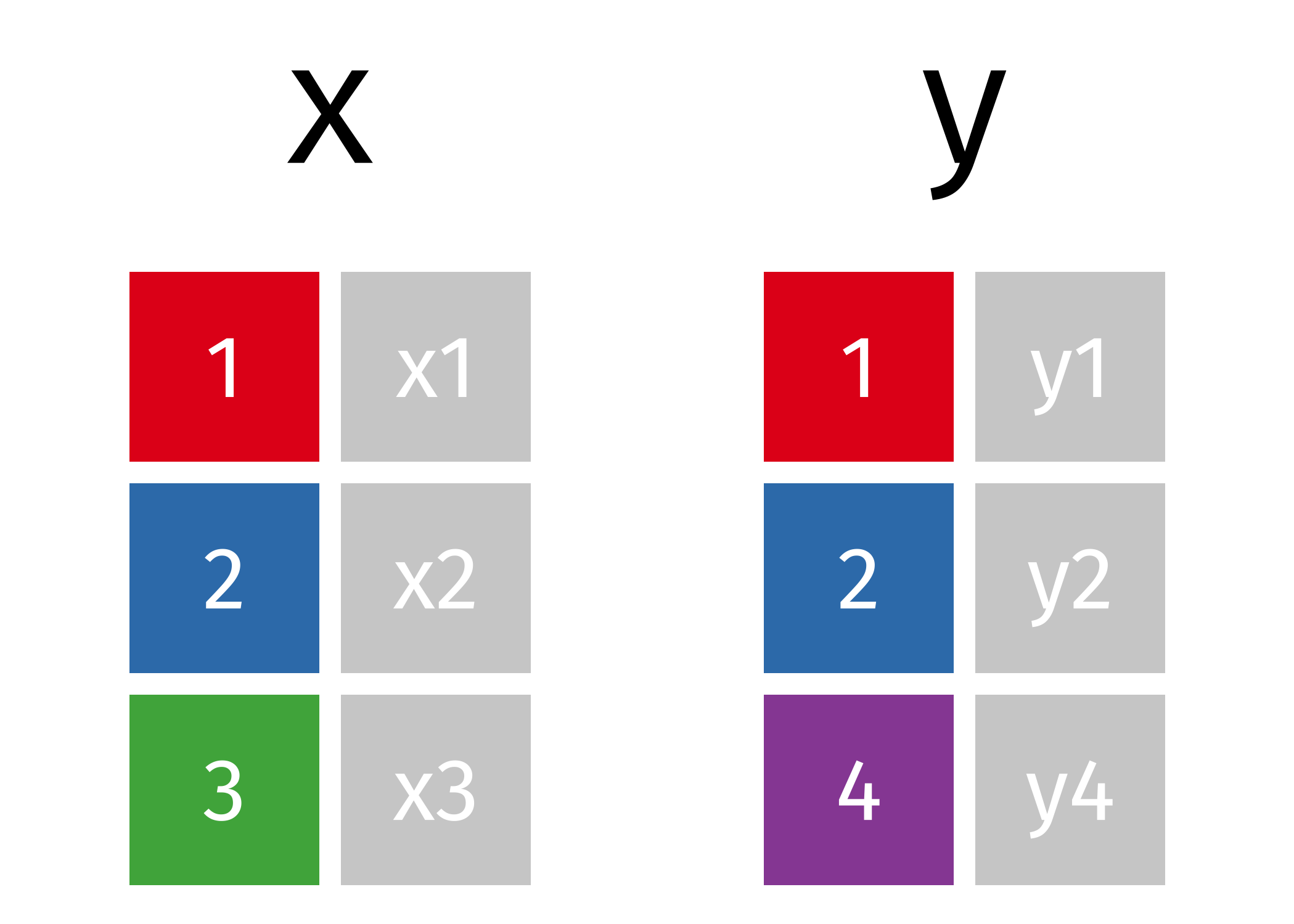
Let’s start with two simple data frames that have one shared column indicating a shared ID:
The first join we will look at is an inner_join(). This function takes two data frames as input and
merges them based on their shared column. Only rows with data in both data frames are kept.

The opposite of an inner_join() is a full_join(). This function keeps all rows from both data
frames, filling in any missing data with NA.
The final join we will look at is a left_join(). This uses the first data frame as a reference and
merges in data from the second data frame. Any rows that are in the left data frame but not the right
are filled in with NA. Any rows in the right data frame but not the left are ignored.

For the sake of completeness, there are also functions for a right_join(), semi_join(), and
anti_join(). But we will not go into how they work because they are far less commonly needed than
the three above.
Challenge 2
Create the following two data frames:
df1 <- tibble(sample = c(1, 2, 3), measure1 = c(4.2, 5.3, 6.1))
df2 <- tibble(sample = c(1, 3, 4), measure2 = c(7.8, 6.4, 9.0))
Predict the result of running
inner_join(),full_join(), andleft_join()on these two data frames. Perform the joins to see if you are correct.Solution to Challenge 2
inner_join(df1, df2)Joining with `by = join_by(sample)`# A tibble: 2 × 3 sample measure1 measure2 <dbl> <dbl> <dbl> 1 1 4.2 7.8 2 3 6.1 6.4full_join(df1, df2)Joining with `by = join_by(sample)`# A tibble: 4 × 3 sample measure1 measure2 <dbl> <dbl> <dbl> 1 1 4.2 7.8 2 2 5.3 NA 3 3 6.1 6.4 4 4 NA 9# df1 as left data frame left_join(df1, df2)Joining with `by = join_by(sample)`# A tibble: 3 × 3 sample measure1 measure2 <dbl> <dbl> <dbl> 1 1 4.2 7.8 2 2 5.3 NA 3 3 6.1 6.4# df2 as left data frame left_join(df2, df1)Joining with `by = join_by(sample)`# A tibble: 3 × 3 sample measure2 measure1 <dbl> <dbl> <dbl> 1 1 7.8 4.2 2 3 6.4 6.1 3 4 9 NA
By default, the join functions will join based on any shared column names between the two data
frames (here just the sample column). You may have noticed the helpful message providing information
about how the join was performed: Joining, by = "sample". You can control which columns are used
to merge with the by argument.
full_join(df1, df2, by = c("sample"))
# A tibble: 4 × 3
  sample measure1 measure2
   <dbl>    <dbl>    <dbl>
1      1      4.2      7.8
2      2      5.3     NA
3      3      6.1      6.4
4      4     NA        9
This may be useful if the data frames share a number of column names, bu only some of them should be
used for merging. You can also use it to merge on a column even if the names don’t match between the
data frames. In this case you need to specify by = c("left_name" = "right_name"):
df3 = tibble(ID = c(1, 2, 4), measure3 = c(4.7, 3.5, 9.3))

# Can't do it automatically
full_join(df1, df3)
Error in `full_join()`:
! `by` must be supplied when `x` and `y` have no common variables.
ℹ Use `cross_join()` to perform a cross-join.
# name in df1 is "sample", name in df3 is "ID"
full_join(df1, df3, by = c("sample" = "ID"))
# A tibble: 4 × 3
  sample measure1 measure3
   <dbl>    <dbl>    <dbl>
1      1      4.2      4.7
2      2      5.3      3.5
3      3      6.1     NA
4      4     NA        9.3
Realistic data
For a more realistic example of joins, let’s turn back to the gapminder data. We have some additional data on countries sex ratios that you should download and save to your data folder.
Read it in and let’s join it to our existing data.
gapminder_sr <- read_csv("data/gapminder_sex_ratios.csv")
Rows: 1722 Columns: 3
── Column specification ───────────────────────────────────────────────────────────────────────────────────────────────────────────
Delimiter: ","
chr (1): country
dbl (2): year, sex_ratio

ℹ Use `spec()` to retrieve the full column specification for this data.
ℹ Specify the column types or set `show_col_types = FALSE` to quiet this message.
gapminder_sr
# A tibble: 1,722 × 3
   country     year sex_ratio
   <chr>      <dbl>     <dbl>
 1 Burundi     1952      91.9
 2 Comoros     1952      98.8
 3 Djibouti    1952      98.6
 4 Eritrea     1952      98.2
 5 Ethiopia    1952      98.6
 6 Kenya       1952     102.
 7 Madagascar  1952     106.
 8 Malawi      1952      92.3
 9 Mauritius   1952      99.2
10 Mozambique  1952      95.6
# ℹ 1,712 more rows
Challenge 3
Which columns are shared between
gapminderandgapminder_sr?.Compare the output of
left,fullandinnerjoins for these two datasets. You may notice that it is possible to join on multiple columns. For example:full_join(gapminder, gapminder_sr)What are the differences between these three joins? What causes these differences?
Solution to Challenge 3
The two datasets share the
countryandyearcolumns.The output from
full_joinhas the most rows, because it is keeping all the rows from both dataframes.inner_joinis only including those rows that match. and has the least rows. Theleft_joinoutput will depend on which data frame was provided first and has the same number of rows as that data frame.
Key Points
bind_rowscombines datasets that share the same variablesThe
joinfamily of functions provide a complete range of methods to merge datasets that share common variables