Introduction to R Markdown

Overview

Teaching: 30 min
Exercises: 40 min

Questions

• What is Markdown/R Markdown?

• How do I turn an R Markdown file into a report?

Objectives

• To understand how R Markdown files are written.

• To integrate text descriptions with code and outputs.

• To adjust parameters that customise a report’s appearance

How does it all work?

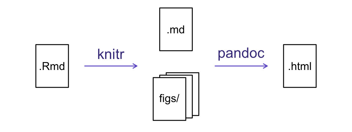
The key R package is knitr. It allows you to create a document that is a mixture of text in Markdown format and chunks of code. When the document is processed by knitr, the chunks of code will be executed, and graphs or other results inserted into an intermediate document.

This intermediate document (all in Markdown format) is then processed by the tool pandoc, which converts it into an html file, with any figures embedded.

Creating an R Markdown file

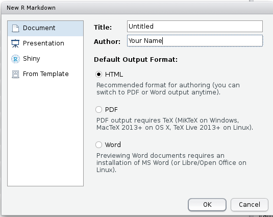
Within RStudio, click File → New File → R Markdown and you’ll get a dialog box like this:

You can stick with the default output (HTML), but give it a title.

R Markdown Metadata

The initial chunk of text (header) contains instructions for R to specify what kind of document will be created, and the options chosen. If you provide no additional information, your header will look pretty slim:

---
title: "Untitled"
output: html_document
---

But you can use the header to give your document a title, author, date, and tell it that you’re going to want to produce html output (in other words, a web page).

---
title: "A Useful Title"
author: "Your Name"
date: "Today's date"
output: html_document
---

Setting up

• Create a new RStudio Project for learning about R Markdown and initialise it with a Git repository
• Create a new R Markdown file in the project.
• Delete all the text after the header block (after the second ---)
• Make sure your document has an appropriate title, author, and date.
• Save and commit your .Rmd file
• Click the Knit button to create your document

Once you click the Knit button , your document will be converted from an R Markdown file into a Markdown file, and then into an html file. A window will also open up to show you a preview of the output.

Since we have not yet written any content for our document, it is obviously looking somewhat bare.

Markdown formatting

Markdown is a system for writing web pages by marking up the text much as you would in an email rather than writing html code. The marked-up text gets rendered to html, replacing the marks with the proper html code.

Structuring content

You can make section headers of different sizes by initiating a line with some number of # symbols:

# Title
## Main section
### Sub-section
#### Sub-sub section

When rendered, this text would be presented as headings that help break up content areas of your writing. For example, The “Markdown formatting” heading above is at the “Main section” level, while the “Structuring content” heading is at the “Sub-sub section” level.

Formatting text

You can format text in a number of ways

You make things bold using two asterisks, like this: **bold**, and you make things italics by using underscores, like this: _italics_. To format text as code, you wrap it in backticks, like this: `code`.

To make a bulleted list you write a list with asterisks or hyphens, like this:

* bold with double-asterisks
* italics with underscores
* code-type font with backticks

or like this:

- bold with double-asterisks
- italics with underscores
- code-type font with backticks

Each will appear as:

• bold with double-asterisks
• italics with underscores
• code-type font with backticks

You can use whatever method you prefer, but be consistant. This maintains the readability of your code.

You can make a numbered list by just using numbers. You can even use the same number over and over if you want:

1. bold with double-asterisks
2. italics with underscores
3. code-type font with backticks

or

1. bold with double-asterisks
1. italics with underscores
1. code-type font with backticks

Will appear as:

1. bold with double-asterisks
2. italics with underscores
3. code-type font with backticks

To aid the readability of your code in text form you should probably use the first options, but again what is important is that you pick one method and stick with it for the entire document.

More Markdown features

You can make a hyperlink like this: [Link to these notes](https://csiro-data-school.github.io/rmarkdown/).

Which appears as: Link to these notes

Including an image file is the same, adding an initial !: !["Image caption"](http://url/for/file). The link for this can either be to an image location on the web, or a file path on your computer.

You can do subscripts (e.g., F₂) with F~2~ and superscripts (e.g., F²) with F^2^.

To include footnotes, use the following format:

Sentence that requires a footnote [^1].

[^1]: Footnote text

The footnote text can be written anywhere in the document and will be shifted to the end when it is rendered into an html page.

Writing text

Add some Markdown formatted text to your document. Make sure to include some section headers, bold and italicised text, and at least one list.

Save and Knit your document. Does it look how you were expecting?

Integrating code

The real power of Markdown comes from mixing markdown with chunks of code. This is R Markdown. When processed, the R code will be executed; if they produce figures, the figures will be inserted in the final document.

The main code chunks look like this:

```{r load_data}
gapminder <- read.csv("data/gapminder.csv")
```

That is, you place a chunk of R code between ```{r chunk_name} and ```. You should give each chunk a unique name, as they will help you to fix errors and, if any graphs are produced, the file names are based on the name of the code chunk that produced them.

To insert a new code chunk into your document, you can use the “Insert” button or the keyboard shortcut Ctrl+Alt+I (Cmd+Opt+I on a Mac).

Writing code

Make sure you have a copy of the gapminder data available. Then write a code chunk to:

• Load the tidyverse package
• Read in the gapminder data
• Filter down to just the Australian data and print it to the screen
• Show a plot of the Australian population over time

Save and Knit your document when you have finished.

You can have as many code chunks as you wish in an R Markdown document. They will all be run in the same environment, so can share variables between them. This allows you to break your code up so that the outputs appear near the relevant text in your document.

Breaking it up

Put your code into three chunks. One for initialisation, one for data minipulation, and one for plotting.

Save and Knit your document when you have finished.

Chunk options

There are a variety of options we can set that control how the code chunks are treated and how their output is produced. A full list of options can be found at the knitr site, but here are some common examples:

• eval controls if the code chunk is actually run.
• echo controls if the code itself is shown in your document.
• results controls how the outputs from your code are shown.
• warning and message can be used to show/hide and warnings or messages produced by your code.
• fig.height and fig.width control the size of the figures produced (in inches).

These options are added in the chunk header, separated by commas. So you might write:

```{r load_libraries, echo=FALSE, message=FALSE}
library("tidyverse")
```

to load the tidyverse package, but not show this code or the message it produces in the final document.

Finer control

For each of your three code chunks, decide if you need to run the code (eval), show the code (echo), show any messages (message), and show the code outputs (results).

Set the relevant chunk options based on your choices (all of these options default to TRUE).

Change the fig.height and fig.width options for the plotting chunk to get a plot that fits in well with the rest of your document.

Global options

Often there will be particular options that you’ll want to use repeatedly; for this, you can set global chunk options, like so:

```{r global_options}
knitr::opts_chunk$set(message=FALSE, warning=FALSE, echo=FALSE, fig.width=11)
```

Changing everything

Use chunk options to control the size of a figure and to hide the code.

Inline code

You can make any part of your report reproducible by using inline code. Use `r and ` for an in-line code chunk, like so: `r mean(some_numbers)`. The code will be executed and replaced with the value of the result.

Don’t let these in-line chunks get split across lines.

If the inline part of the code would otherwise be too long, perhaps precede the paragraph with a larger code chunk that does calculations and defines variables. This code chunk can be hidden by setting the echo=FALSE and results=FALSE options, but the variables can then be referenced using an inline code chunk in the following paragraph.

Coding inline

Add a sentence at the bottom of your document that shows the versions of the software used to create it. Using inline code sections, describe which version of R and the tidyverse package you are using by calling getRversion() and packageVersion("tidyverse").

Key Points

• Markdown is a way of writing text files in a structured way.

• R Markdown allows integration of R code with Markdown.

• Chunk options can be used to control formatting.