```{r setup, include = FALSE}
knitr::opts_chunk$set(
results = 'asis',
warning = FALSE,
message = FALSE,
fig.align = 'center'
)
#Load libraries
library(tidyverse)
library(readxl)
library(kableExtra)
library(knitr)
```
# Introduction
My name is Melania Figueroa and I am currently Leader of the Next Generation Crop Protection Group, Ag & Food Traits Program. I am very interested in understanding the evolution of rust fungi and delivering genetic disease resistance to cereals. I did not have any previous experience using R language before Data School.
# My Project
I aim to identify genes responsible for virulence in rust fungi. In this case, our team is asking if deletions of specific genes (effectors) result in gain of virulence in a species of fungus (_Puccinia graminis_). Here, I am visualising data that depicts gene coverage in a defined region of the genome of _P. graminis_.
{width=300px}
# Data used in this project
My project uses two dataframes called: `read_coverage_AvrSr27_deleted.xlsx` and `Phenotypes.xlsx`.
I am sharing here code to input and read dataframes
```{r reading dataframes}
#Step 1. Read in dataframes and assign them to objects
Del_pgt21 <- read_excel("data/read_coverage_AvrSr27_deleted.xlsx")
Phenotypes <- read_excel("data/Phenotypes.xlsx")
```
Here is preview of dataframe `Del_pgt21`
```{r Del_pgt21, out.width='100%', echo = FALSE}
knitr::kable(head(Del_pgt21, n = 5), format = "html") %>%
kable_styling("striped")
```
and a preview of dataframe `Phenotypes`
```{r review Phenotypes, out.width='100%', echo = FALSE}
knitr::kable(head(Phenotypes, n = 5), format = "html") %>%
kable_styling("striped")
```
Some scripts to manipulate dataframes and prepare materials for plotting are included below.
It was key to extract the data I cared about (only certain strains) and so I created a different table, `Del_pgt21`
```{r extracting relevant data }
#Step 2. The dataframe _Del_pgt21_ has more information than I needed so I #extracted the data for the rust strains I care about. Here I created a new #dataframe called *gcoverage_isolate*:
gcoverage_isolate <- Del_pgt21 %>%
select("ID","21-0,percent zero bases",
"Sr27_1,percent zero bases","Sr27_2,percent zero bases",
"Sr27_3,percent zero bases", "34M1,percent zero bases",
"34M2,percent zero bases", "98,percent zero bases",
"194,percent zero bases", "SA01,percent zero bases",
"SA02,percent zero bases","SA03,percent zero bases",
"SA04,percent zero bases", "SA05,percent zero bases",
"SA06,percent zero bases", "SA07,percent zero bases")
```
Then, I was set up to tidy my data in `Del_pgt21`.
```{r tidy dataframe gcoverage_isolate}
#*Step 3. Tidy the dataframe _gcoverage_isolate_:
tidy_gcoverage_isolate <- gcoverage_isolate %>%
gather(key = "Percent_coverage", value = "coverage", -ID)
```
Another task was to manipulate column names and other content of the dataframes so I could get ready to make some plots.
```{r adjusting gene coverage values}
#Step 4. Complete other dataframe manipulations.
#In the column "Percent_coverage", the isolate name was combined with other #information, for example"21-0,percent zero bases", so I separated this using the #"," . The dataframe was also showing "0" to indicate full coverage so I changed #this to make it "100". Here, I created a new dataframe called *df_plot*.
df_plot <- separate(tidy_gcoverage_isolate,
Percent_coverage, into = c("isolate","percent"), sep = "," ) %>%
mutate(Coverage = 100-coverage) %>%
select(-"percent", - "coverage")
#Some rust strains mentioned in the _tidy_gcoverage_isolate_ dataframe needed renaming becuase they did not match the information provided by the dataframe _Phenotypes_. Here, I created another dataframe called *df_plot2*
df_plot2 <- df_plot %>%
mutate(isolate = str_replace(isolate,"Sr27_", "Mutant ")) %>%
mutate(isolate= str_replace(isolate,"SA", "SA-")) %>%
mutate(isolate = replace(isolate, isolate == "194", "194-1,2,3,5,6")) %>%
mutate(isolate = replace(isolate, isolate == "98", "98-1,2,3,5,6")) %>%
mutate(isolate = replace(isolate, isolate == "34M1", "34-2-12")) %>%
mutate(isolate = replace(isolate, isolate == "34M2", "34-2-12-13"))
#I converted the columns to factors becuase otherwise the plot won't mantain the order of genes and isolates that I wish to keep from the daaframe.Here, I created another dataframe called *df_plot3*
df_plot3 <- df_plot2 %>%
mutate(isolate = factor(isolate,levels = rev(unique(isolate)))) %>%
mutate(ID = factor(ID,levels = unique(ID)))
```
Next, I started working with the dataframe `Phenotypes`, which provides information about phenotypes, to then integrate with the data about deletions of genes in the region of interest. So, manipulations in this dataframe began.
```{r}
#Here, I needed to fix the column name to be Sr_gene
colnames(Phenotypes)[1] <- "Sr_gene"
#Then I prepared a tidy dataframe and clarified the information in the column"reaction", otherwise the data was going to be difficult to be interpreted. The dataframe created here was named *clean_phenotypes*.
clean_phenotypes <- Phenotypes %>%
gather(- Sr_gene, key = "isolate", value = "reaction") %>%
mutate(reaction = replace_na(reaction,"N")) %>%
mutate(reaction = replace(reaction, reaction == "?", "N")) %>%
mutate(reaction = replace(reaction, reaction == "A/V", "N")) %>%
mutate(reaction = replace(reaction, reaction == "A", "Avirulence")) %>%
mutate(reaction = replace(reaction, reaction == "V", "Virulence")) %>%
mutate(reaction = replace(reaction, reaction == "X", "Mesothetic")) %>%
mutate(reaction = replace(reaction, reaction == "N", "Unknown")) %>%
mutate(isolate = factor(isolate,levels = unique(isolate)))
#The column order needed to be changed to make it easier to read and then the phenotypes of the rust strains when gene Sr27 is present in the plant was extracted since it was the only bit of data I cared about. Here, I finished with a dataframe called *pheno_interest*
clean_phenotypes <- clean_phenotypes[c(2,1,3)]
pheno_interest <- clean_phenotypes %>%
filter(Sr_gene =="27")
```
After tidying and extracting the data I needed, I joined the two tables by isolate name.
```{r linking data from two tables}
#*Step 6. Next I needed to link up the data regarding phenotypes for Sr27 and #gene coverage that reflects deletions. Here, I created a new dataframe called:
#*df_plot4*.
df_plot4 <- right_join(pheno_interest, df_plot3, by = "isolate")
```
## Data visualisation
Now, we have all the elements to make some plots and visualise our data
```{r first plot}
del_heatmap <- ggplot(data = df_plot3,
mapping= aes(y=isolate, x= ID, color = Coverage)) +
geom_tile(aes(fill = Coverage), color="white") +
theme_minimal() +
theme(text = element_text(size=8),
axis.text.x = element_text(angle=90, hjust=0.1,vjust=0.1, color= "black"),
axis.text.y = element_text(angle=0, hjust=1,vjust=1, color = "black")) +
ylab("Isolate") +
xlab("Gene model") +
scale_fill_gradient(low = "lightgray", high ="red") +
scale_x_discrete(expand = c(0, 0),
position = "top") +
coord_equal()
```
and I ended up with something like this:
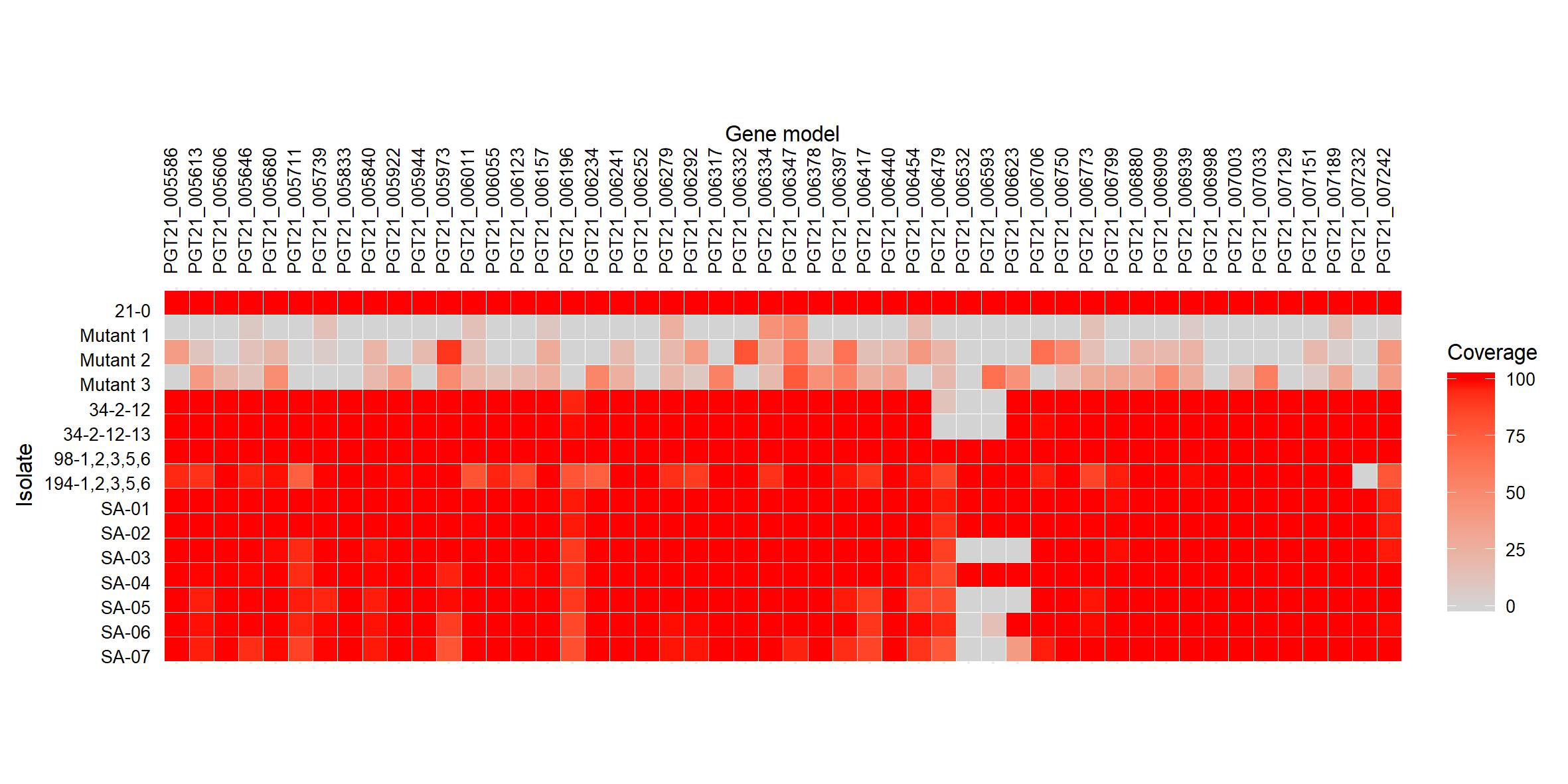{width=600px}
I saved my plot using the code below, although the phenotypic data was yet to be included.
```{r saving first plot}
ggsave("results/deletion_heatmap.jpg", plot = del_heatmap,
width = 20, height = 10, units = "cm")
```
Then I re-did this plot but showing the isolates that are virulent or avirulent on wheat that carry the gene Sr27 modifying my code as follows
```{r}
heatmap_2 <- df_plot4 %>%
mutate(isolate = factor(isolate,levels = rev(unique(isolate)))) %>%
ggplot(
mapping= aes(y=isolate, x= ID, color = Coverage)) +
geom_tile(aes(fill = Coverage), color="white") +
theme_minimal() +
theme(text = element_text(size=10),
axis.text.x = element_text(angle=90, hjust=0.1,vjust=0.1, color= "black"),
axis.text.y = element_blank(),
panel.grid = element_blank()) +
ylab("Isolate") +
xlab("Gene model") +
scale_fill_gradient(low = "lightgray", high ="red") +
scale_colour_manual("Virulence", values= c("grey70","black")) +
scale_x_discrete(expand = expand_scale(mult = c(0, 0), add= c(7,0)),
position = "top") +
coord_equal() +
geom_text(aes(x = 0, y = isolate, label = isolate, colour = reaction), hjust = 1, size = 3)
ggsave("results/phenotype_heatmap.jpg", plot = heatmap_2,
width = 20, height = 16, units = "cm")
```
And here I can show you my final plot
{width=800px}
# My Digital Toolbox
Since starting data FOCUS school I have learned:
* `dplyr`, `ggplot`, `R markdown`
# My time went ...
to tidying the data. This was the most difficult part. It was surprising how many name inconsistencies existed between the two tables. This made it hard to combine information from both tables to generate a hypothesis.
# Next steps
I did not have time to apply statistics to determine if the deletion of one or more genes could explain the change in phenotype. So, I would like to explore this question further, and apply some other material we covered in the course.
# My Data School Experience
Data School has been a very positive experience and has made me aware of the many resources we have access to enhance computational skills within our groups. This small project is part of a publication my group is working on. I am keen on gaining additional expertise to bring those to my group. My experience will benefit memeber of my groups as I will be better possition to guide them through data management practices.
This document was completed using R `r getRversion()` and the tidyverse package `r packageVersion("tidyverse")`
{width=100px}{width=100px}{width=100px}
{width=100px}